tufazip: Learning to Compress a Billion Bytes of Wikipedia

Summary

I took #2 on the Large Text Compression Benchmark,Large Text Compression Benchmark (Matt Mahoney). (at the time of submission: Sept. 7, 2026) a benchmark that has been running for 20+ years, with tufazip, the best-performing entry using a neural network as its sole prediction model. My final result compressed one billion bytes of Wikipedia into 105,388,353 bytes (105.39 MB), including the offline trained weights and decoder.

The final system uses a 12-layer, 163M-parameter Transformer, initialized from a 34M-parameter offline model quantized to 4.33 MB. Two offline trained layers are copied into twelve independent layers, which continue learning as the file is compressed. The decoder repeats the same learning process, so the full model’s learned weights never need to be transferred.

Introduction

What is intelligence? Broadly speaking, intelligence is typically linked to capability of abstraction, logic, reasoning, problem solving, and adaptability; in daily use, we often use it to just mean crystallized intelligence. But it’s not so clear…it’s an age-old question that remains difficult to answer. Let’s look at a few concrete perspectives focused on machine intelligence:

• Achieving goals: Shane Legg and Marcus Hutter define intelligence as “an agent’s ability to achieve goals in a wide range of environments.”Universal Intelligence: A Definition of Machine Intelligence (Legg and Hutter, 2007). Here, Legg and Hutter emphasize the breadth of environments the agent can handle and its ability to accomplish tasks within them.

• Learning new skills efficiently: François Chollet defines intelligence as skill-acquisition efficiency: how effectively a system turns its prior knowledge and experience into new abilities.On the Measure of Intelligence (Chollet, 2019). Think of picking up an unfamiliar game from a few examples. Learnability is still important but with an additional focus on efficiency.

• Finding useful representations: One perspective inspired by Kenneth Stanley’s work is that intelligence depends on finding abstractions that make learning and problem solving easier. Think of discovering a reusable rule that connects several seemingly unrelated problems. Interestingly, Stanley and colleagues argue here that how knowledge is organized inside a system, despite being much more ambiguous to measure, may matter for its ability to generalize and keep learning.Questioning Representational Optimism in Deep Learning: The Fractured Entangled Representation Hypothesis (Kumar, Clune, Lehman, and Stanley, 2025).

• Compressing information: Matt Mahoney argues for understanding intelligence through compression: the ability to capture the structure in observations so they can be described more compactly. For text, learning spelling, grammar, and relationships makes the next word more predictable—and predictable information takes fewer bits to encode. From this perspective, compression gives us a concrete way to measure how much structure a system has captured.Rationale for a Large Text Compression Benchmark (Mahoney, 2009), section “Compression is Equivalent to General Intelligence.”

Inspired by the compression perspective, we focus on lossless compression as our task. For text, the connection between prediction and compression is especially direct. If a model assigns probability $p$ to the next token, its ideal encoding cost is $-\log_2 p$ bits. Doubling the probability assigned to the token that actually occurs saves one bit. For a fixed tokenization, next-token prediction and compression have the same objective: the summed cross-entropy loss in bits is exactly the ideal compressed length.

\[\text{loss} = -\sum_t \log_2 p(x_t \mid x_{<t}) = \text{ideal bits}.\]

Here, $x_t$ is the token at position $t$ and $x_{<t}$ is the preceding text. Arithmetic coding turns this correspondence into a practical compressor, using the model’s probabilities to encode likely tokens with fewer bits and surprising ones with more. This equivalence is explored in more depth by Delétang and colleagues in Language Modeling Is Compression.Language Modeling Is Compression (Delétang et al., 2023). Learning key parts of language such as spelling, grammar, facts, and relationships all help a model anticipate the text and save bits. Empirically on modern language models, Huang and colleagues find in Compression Represents Intelligence Linearly Compression Represents Intelligence Linearly (Huang et al., 2024). that compression of external text closely correlates with average downstream benchmark performance across the language models they study. Compression on one file is a limited measure of intelligence, but it gives us a concrete way to study how well a model captures structure.

This motivation underlies the Hutter Prize,Prize for Compressing Human Knowledge (Marcus Hutter). which rewards lossless compression of Wikipedia. For this project, I used Matt Mahoney’s Large Text Compression Benchmark1 and its billion-byte Wikipedia file, enwik9. I also used enwik8, the first 100 million bytes of enwik9, to compare configurations and select candidates for full enwik9 runs. The benchmark task is to represent the entire billion-byte file as compactly as possible losslessly. Under the benchmark’s scoring rules,Rules for the Large Text Compression Benchmark (Matt Mahoney). the score includes the compressed text plus the zipped decoder containing any information needed for decoding. This makes the cost of an offline trained model part of the problem: better predictions must save more space than an offline model adds.

Text compressors exploit structure in different ways. It helps to distinguish transformation, prediction, and coding: a compressor can first transform the text, then estimate probabilities, then encode likely outcomes with fewer bits. The first step might tokenize the text or reorder its sections, while preserving enough information to reconstruct the original text exactly. The second step estimates probabilities for the next symbol, using anything from counts of earlier patterns to a neural network. The last step uses those probabilities to encode the symbols as bits, with an entropy coder such as an arithmetic coder or a Huffman coder.Data Compression Explained (Matt Mahoney), especially the chapters on coding, modeling, and transforms. Let’s take a brief look through major developments in compressors and how they changed these three stages:1

1. General-purpose foundations: repeated strings and block sorting. Gzip’s DEFLATE format uses the following for the three roles: LZ77 transforms repeated byte sequences into references to earlier occurrences, symbol frequencies provide a simple probability model, and Huffman coding gives common symbols shorter bit strings.GNU gzip overview and DEFLATE format specification, RFC 1951 (Deutsch, 1996). Bzip2 takes another route at the transformation stage, using the Burrows–Wheeler transform to group bytes with similar surrounding text. Further transforms make this repetition easier to model, and the coding stage also uses Huffman coding.bzip2 manual (Julian Seward), introduction and algorithm references. These methods exploit repetition and byte statistics without needing an English dictionary or grammar.

2. 1980s–2000s: statistical next-character prediction. PPM, introduced by Cleary and Witten in 1984, focuses on prediction: it counts which characters follow previously seen contexts, falling back to shorter contexts for unseen continuations. These counts supply next-character probabilities to the coding stage, which uses arithmetic coding. The predictor adapts as it reads the file.Data Compression Using Adaptive Coding and Partial String Matching (Cleary and Witten, 1984); Mahoney’s PPM explanation describes the context counts and escape mechanism. Here, learning from the input was already key, even though the predictors were statistical tables.10

3. 2000s: context mixing. The PAQ family expanded the prediction stage to combine models using different clues, including recent bytes, whole words, and long matches. PAQ7 and PAQ8 used neural networks to mix their predictions into a probability for the next bit. The coding stage then used that probability to arithmetic code the actual next bit.The PAQ Data Compression Programs (Matt Mahoney), with model histories in Data Compression Explained. PAQ8h led enwik9 when the Hutter Prize launched in August 2006.1

4. 2006: text-specific preprocessing was already important. XML-WRT improved the transformation stage: it replaced common words and XML fragments with compact symbols before passing them to a predictor and coder, such as those in PPM. The PAQ8HP entries also used dictionary transforms: words became short codes, while markers preserved capitalization. Some versions grouped dictionary words by grammatical or semantic similarity. These reversible transformations changed what the downstream models had to predict; the coding stage still encoded those symbols using the predicted probabilities. Note the required dictionaries counted toward the compressed size as an offline calculated prior.The benchmark’s XML-WRT and PAQ8HP descriptions document their transforms, dictionary organization, and dictionary-inclusive results.

5. 2014–2019: larger ensembles and LSTM predictors. Byron Knoll’s cmix, first released in 2014, expanded the prediction stage with more predictors and a larger mixing network, while using text preprocessing for transformation.cmix (Byron Knoll), release history and architecture description. It included an LSTM by 2016. In 2017, Knoll’s lstm-compress kept the preprocessing but removed the other predictors, leaving the LSTM to model the sequence.See the cmix and lstm-compress entries in the benchmark, and Knoll’s lstm-compress description. Bellard’s NNCP followed in 2019: a subword preprocessor transformed the text for its larger models, neural networks predicted the resulting symbols, and arithmetic coding encoded them using those probabilities.Lossless Data Compression with Neural Networks (Bellard, 2019).

6. 2021–2023: Transformers and replay. Bellard had tested Transformers in 2019, but they initially compressed worse than his LSTMs.18 NNCP v2 surpassed cmix on enwik9 in 2021 by strengthening the prediction stage with an improved Transformer and replay: periodically training again on earlier text. Preprocessing still handled transformation, and arithmetic coding used the predictor’s probabilities to encode the symbols. The encoder and decoder repeated the same learning, so the learned weights did not need to be transferred.NNCP v2: Lossless Data Compression with Transformer (Bellard, 2021). By 2023, NNCP v3.2 reached 107.26 MB, including its decoder bundle.1

7. 2026: hybrid systems and automated research. Recent entries combine elaborate transformations with hybrid predictors that mix compact neural models and statistical models. fx2-cmix-transformer uses a 6M-parameter, offline trained Transformer with four-bit weights alongside PPMd and context mixing, retaining text preprocessing and arithmetic coding.fx2-cmix-transformer writeup (Vladimir Ivanov, 2026). cmix-neif combines a Transformer, an online LSTM, and statistical models in its prediction stage, while improving transformation through changes to article ordering and metadata handling.cmix-neif description (Marcus Wölk, 2026). Alongside these entries, automated research is emerging: an enwik8 collaboration uses autonomous LLM agents to explore transformations and predictors, run experiments, and share results. Compression supplies a concrete score for this research loop: propose a change, measure its effect, and iterate.Compression is Intelligence: agent collaboration on enwik8. The separate cm autoresearch project also lets agents modify a compressor and score their changes on a fixed corpus.

For me personally, as an AI researcher, I wanted to explore how far a simple Transformer could go as the sole predictor. The result is tufazip. Its predictor is a 12-layer, 163M-parameter decoder-only Transformer consisting of a self-attention sublayer and a feed-forward MLP sublayer. The architectural choices include rotary position embeddings (RoPE), SwiGLU MLPs, RMSNorm before and after each attention and MLP sublayer, and normalization of attention queries and keys. The final output assigns a probability to each possible next token. Starting from NNCP, I improved the model and training recipe to reach 105.98 MB using online learning alone, then reduced that to 105.39 MB with an offline trained prior, including the weights and decoder. tufazip took #2 (at the time of submission: Sept. 7, 2026) on the Large Text Compression Benchmark and became the best-performing entry using a neural network as its sole prediction model.

Tufazip: Learn without transferring the weights (and later offline transfer)

tufazip combines a Transformer predictor with an arithmetic coder. The text is converted reversibly into tokens, and the Transformer assigns probabilities to the next token using text already known to the decoder.

Arithmetic coding turns those probabilities into a compressed stream. Conceptually, it starts with an interval from zero to one, divides it into pieces proportional to the next-token probabilities, and keeps the piece corresponding to the actual token. Repeating this process narrows the interval; the compressed bits identify a point inside it. More probable tokens leave wider intervals, requiring fewer bits. The decoder uses the same probabilities to reverse these choices and recover the tokens. The final compressed artifact is a number between zero and one. 10

Figure 1. Four symbols—A, B, C, and an end marker—have probabilities 0.6, 0.2, 0.1, and 0.1. The highlighted ranges encode A → C → end. Each row zooms into the selected range; the dot marks the encoded value. `tufazip` updates these probabilities as it learns with gradient descent.Arithmetic encoding diagram by Dcoetzee (2007), released into the public domain.

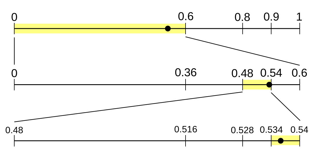
For the online run, the encoder and decoder start from identical randomly initialized weights and repeat the same learning process:19

1. Predict: both models produce the same next-token probabilities from the text they already know.
2. Encode or decode: the encoder writes the actual token using those probabilities; the decoder recovers it from the compressed stream.
3. Learn: now that both sides know the token, they perform the same training update before making further predictions.

The decoder therefore reconstructs the online training of the model as it reconstructs the text. Notably, the weight update from learning and next-token probabilities must be fully deterministic in order for the algorithm to be lossless. The weights learned online never need to be transferred.

We also explored offline transfer: train a compact model in advance, transfer it, and then continue to learn online. The decoder is initialized with the transferred weights and then learns online as before. This gives the model a trained starting point, but introduces a storage cost: the initialization must save more compressed text than it adds.

Ablations: What actually helped?

We do ablations to understand which parameters are crucial to the model’s performance - in this section we focus on replay, vocabulary, and parameter count.

Replay gives the model more opportunities to learn by Periodically revisiting a window of earlier text and performing additional training. All of that text has already been decoded, so replay requires no additional training data in the archive. We find replay consistently improves later predictions, at the cost of more computation during both compression and decompression.19 Vocabulary defines the tokenizer used to tokenize the text losslessly before training on the tokens, and model size gives the size of the neural network used for prediction and training. Smaller vocabularies consistently helped, while and larger models had less consistent trends. For the results, all sizes below use decimal MB; payload means the compressed data, while total also includes the decoder and its required files.

Replay

Consistently, a larger replay helped at a large computation cost. With the same 163M-parameter model and 4K vocabulary, increasing the replay window from 15M to 35M tokens reduced the full enwik9 payload from 107.22 to 105.92 MB. That saved 1.30 MB, or 1.21%, for about 40% more estimated model FLOPs: 7.45 × 10¹⁹ to 1.04 × 10²⁰ operations, including online learning and replay.

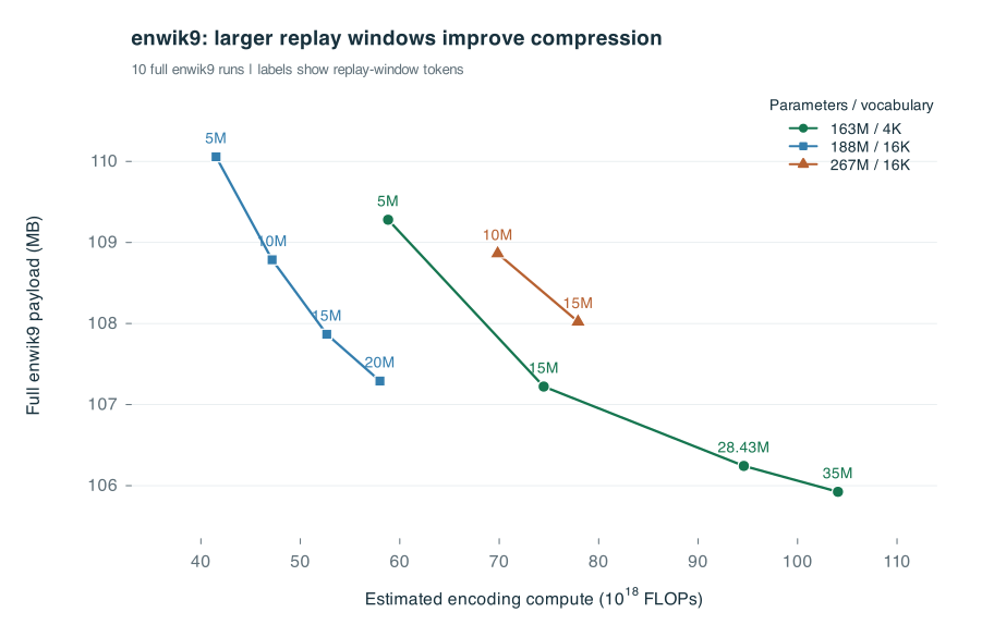
Figure 2. Replay-window ablations: ten full enwik9 runs. Each line holds the model and training recipe fixed while varying window size. Labels show replay-window tokens.

Vocabulary

Consistently, a smaller vocabulary helped. In a comparison with 5M-token replay, the 4K word tokenizer beat both 8K and 16K. Surprisingly, Dedicated XML/wiki tokens made compression worse, despite the abundance of markup in the input. This compares complete tokenizer configurations: changing tokenization also changes how much source text fits into a fixed number of context or replay tokens.

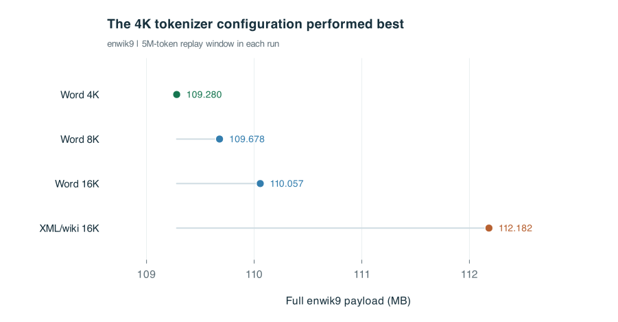
Figure 3. Tokenizer comparison on enwik9, using a 5M-token replay window. Lower is better.

Parameters

More parameters did not help in the matched enwik9 comparisons. With a fixed 16K vocabulary, the 267M model produced slightly larger payloads than the 188M model at both 10M and 15M replay windows. On enwik8, a separate sweep with a fixed 4K vocabulary and 15M-token replay window showed gains from 14M to 77M parameters. Compression changed little at 163M and worsened at 336M. We hypothesize that on compressing a fixed text document, there is an optimal model size where the payload gets bigger when using a smaller or larger model.

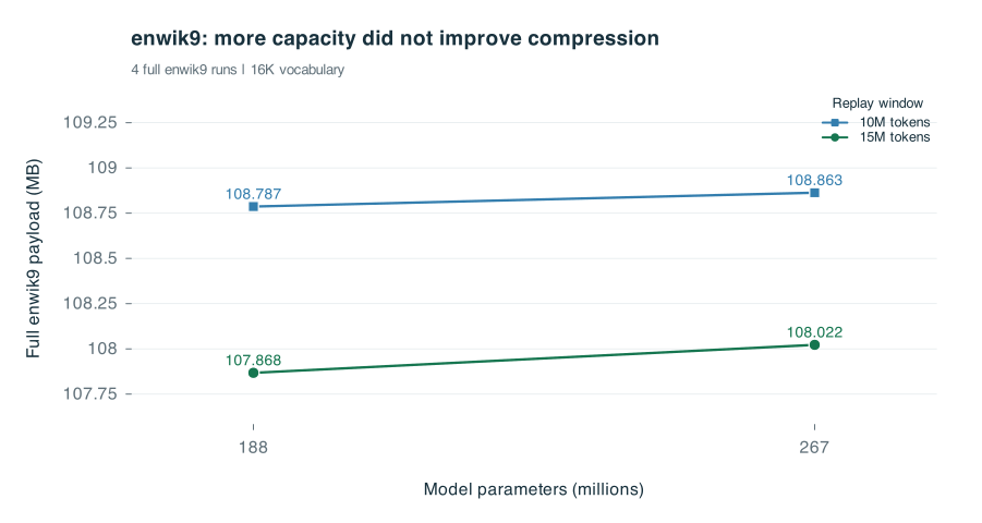
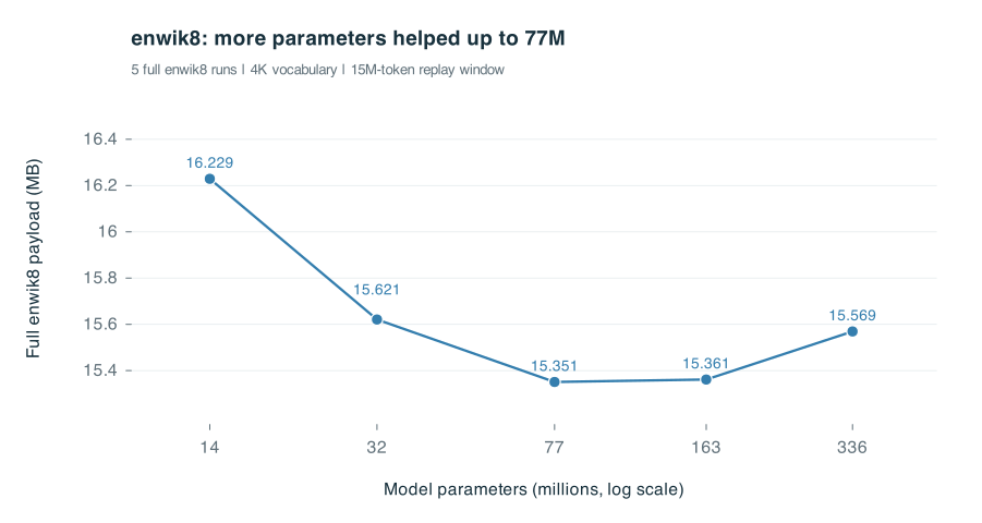
Figure 4. Model capacity across four full enwik9 runs (top) and five full enwik8 runs (bottom). Each line holds the training recipe and replay window fixed while varying model size.

Our Best Online Run

Our best online run used a 12-layer, 163M-parameter Transformer with a 4K word vocabulary, 192-token context, 35M-token replay window, and 0.25 replay dropout. It compressed the full enwik9 to 105.92 MB of payload, or 105.98 MB including the decoder (0.848 bits per byte). This is the online baseline for the offline-transfer experiments below.

Offline transfer: Can offline trained initialization pay for itself?

Online learning avoids transferring weights, but it starts without a trained model. Could offline training give it a useful head start? We explored several model families for the prior:

• Full-precision models: provide an empirical lower-bound reference for compressed-text size before quantization, using models from 14M to 336M parameters on enwik8 and 96M to 367M on enwik9.
• Dense low-bit models: retain independent Transformer blocks while storing their weights at uniform or mixed low precision.
• LoRA and quantized LoRA (QLoRA): add small, low-rank corrections to a quantized model. Both the base model and the corrections count toward the total; our quantized LoRA variant stores the corrections at four bits.
• Compact architectures expanded online: vary stored depth across 3, 6, 9, and 12 layers, or share blocks across depth. The shared variants included one repeated block, cycles of two or three blocks, and repeated middle blocks between distinct first and last layers.

We also explored how to train the low-bit priors:

• Quantization-aware training: train with low-precision weights, and vary how many bits different parts of the model receive. We also tested which layers and tensors contributed most to prediction quality.
• Initialization and training recipes: directly quantize offline trained weights, lower precision in stages, train from scratch, or distill predictions from a full-precision teacher.

The table summarizes the model families, with the compact layouts listed individually. Sizes include both the base model and any adapters; compact rows use the one-bit prior budgets for enwik9. In those layouts, each letter denotes a stored Transformer block; · denotes an inserted identity block that initially passes its input through unchanged. Repeated letters share weights offline, then become independent copies online. Each compact layout expands to twelve online layers.

Model family / layout	Explanation	Prior size (MB)
Online baseline	Twelve independent, randomly initialized blocks: ABCDEFGHIJKL	0
Full-precision models	Independent blocks with FP32 weights: 14M, 32M, 77M, 163M, and 336M parameters on enwik8; 96M, 188M, and 367M on enwik9.	enwik8: 55.12–1,342.60 enwik9: 383.98–1,468.47
Dense low-bit models	The five enwik8 model sizes above, with independent blocks and uniform or mixed low-bit weights.	3.53–42.51
LoRA	The same five enwik8 sizes, with a frozen quantized base and low-rank adapters stored at 16 bits.	4.79–53.93
Quantized LoRA (QLoRA)	32M, 77M, 163M, and 336M bases on enwik8; our variant also quantizes the adapters to four bits.	6.34–45.82
Compact: Loop1	One block repeated twelve times: AAAAAAAAAAAA	2.70
Compact: Cycle2 (C2)	Two blocks repeated six times: ABABABABABAB	4.33
Compact: Cycle3 (C3)	Three blocks repeated four times: ABCABCABCABC	5.96
Compact: Middle1 (M1)	Distinct first and last blocks around one repeated middle block: ABBBBBBBBBBC	5.97
Compact: Middle2 (M2)	Distinct first and last blocks around two alternating middle blocks: ABCBCBCBCBCD	7.59
Compact: Three-layer prior (L3)	Three independent blocks plus nine identity blocks: A···B···C···	5.95
Compact: Six-layer prior (L6)	Six independent blocks plus six identity blocks: A·B·C·D·E·F·	10.84
Compact: Nine-layer prior (L9)	Nine independent blocks plus three identity blocks: ABC·DEF·GHI·	15.80
Compact: Twelve-layer prior (L12)	Full depth, with no sharing or inserted blocks: ABCDEFGHIJKL	20.70

Every approach faces the same target:

transferred model + compressed text and decoder < online baseline.

Plotting transferred model size in the x-axis against the compressed text and decoder size in the y-axis shows a green triangle of our target region. Each extra megabyte spent on weights removes one megabyte from the remaining budget. If we can find a result in the green region, then we will have found an offline transfer that beats the online only training, which entail 15.152 MB for enwik8, and 105.979 MB for enwik9, respectively.

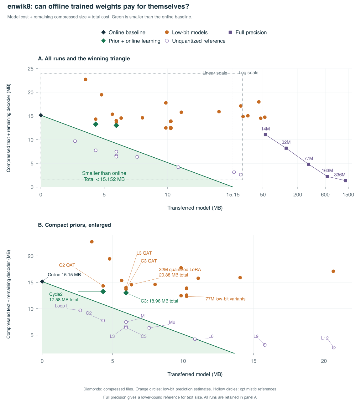
Figure 5. On enwik8, the tested transferred priors remained outside the winning region. Strong unquantized predictions were difficult to preserve within the storage budget.

The upper plot includes all runs: the x-axis stays linear through the winning triangle, then switches to a logarithmic scale. Full-precision squares show prediction quality before quantization, with actual stored weight sizes on the x-axis. The lower plot enlarges the compact priors.

Orange circles group the low-bit experiments, including quantization and adapters. Hollow circles pair unquantized prediction quality with a low-bit storage budget as an optimistic reference. Diamonds show compressed file sizes; the other filled points use prediction-based size estimates.

Among the dense quantization and adapter experiments, 32M quantized LoRA had the best estimated total at 20.88 MB. The compact two-block and three-block priors, followed by online learning, reached 17.58 and 18.96 MB. Both still exceeded the 15.15 MB online baseline.

Based on the partial enwik8 results, we chose Cycle2 (C2) and the six-layer prior (L6) to continue on enwik9. The billion-byte file gives a fixed-size prior ten times as much data over which to recover its cost. Here, C2 crossed the boundary.

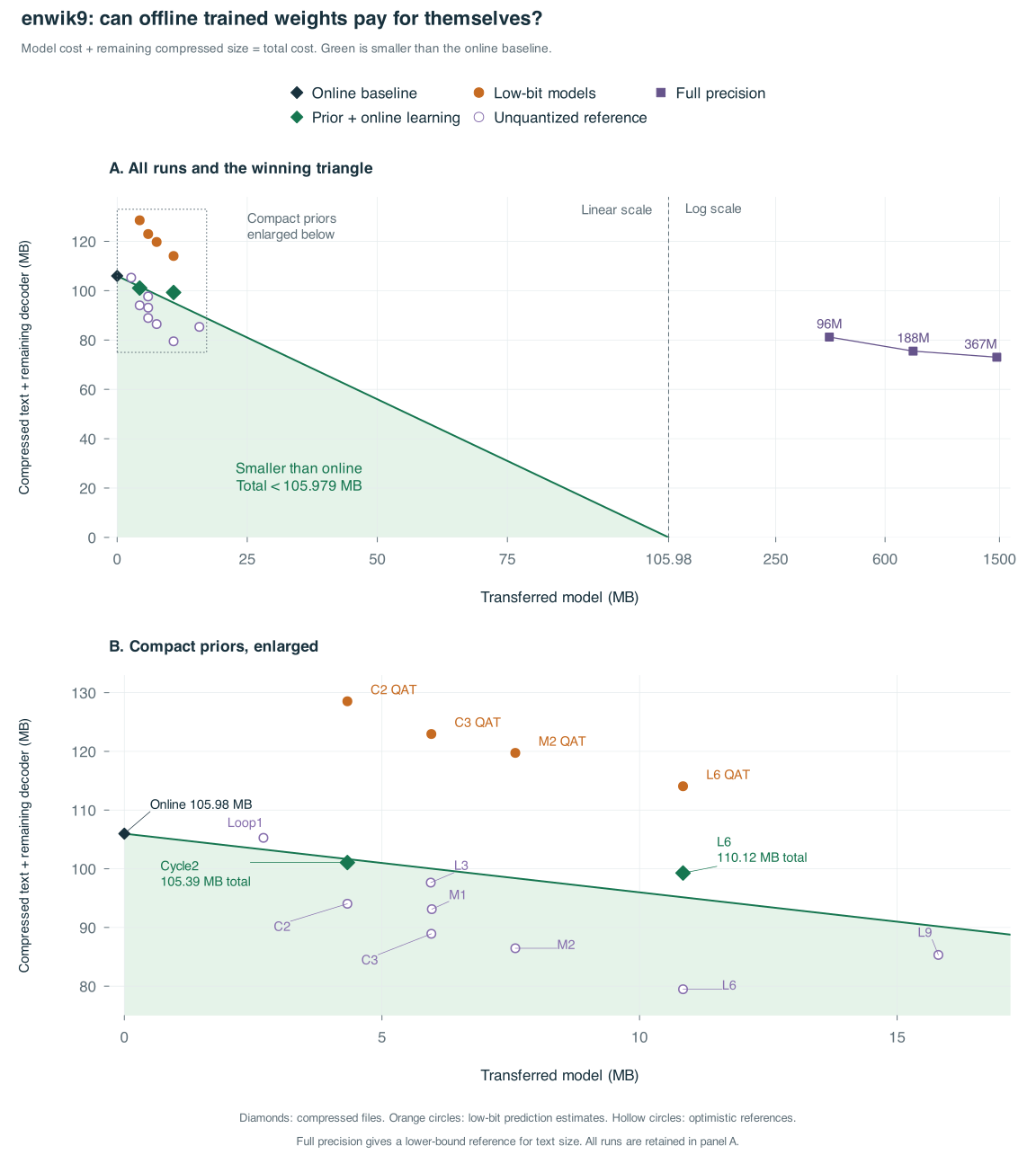
Figure 6. On enwik9, C2 saves enough compressed text to cover its model cost. L6 predicts better, but costs too much to transfer.

The upper plot includes all runs, with a linear x-axis through the winning triangle and a logarithmic scale beyond it; the lower plot enlarges the compact priors. Full-precision squares include actual stored weight sizes. Orange circles show low-bit prediction estimates, hollow circles show optimistic unquantized references at low-bit storage budgets, and diamonds show compressed file sizes.

C2 trains two shared blocks repeated across twelve steps, stores them once each, then copies them into twelve independent layers. Online learning lets those copies specialize without adding to the transferred model. Results from the full enwik9 runs were:

Configuration	Payload MB	Decoder + weights MB	Total MB
Online v1	105.924	0.055	105.979
L6	99.173	10.945	110.118
C2	100.958	4.430	105.388

L6 produced the smaller payload, but its larger weight bundle erased the savings. C2 saved 4.97 MB of payload while adding 4.38 MB of decoder cost, leaving a net improvement of 0.59 MB, or 0.56%, over online v1. We finalized on C2 as the final configuration for tufazip v2, achieving a total compressed size of 105,388,353 bytes (105.39 MB) on enwik9, including the offline trained weights and decoder.

Discussion

Some may question the value of this benchmark in the modern era, I still find this benchmark valuable even in the era of automated research loops. Under the intelligence-as-compression perspective, a smaller complete artifact is evidence that we have found a more intelligent representation of the same corpus. Including the decoder and offline trained weights makes that meaningful: moving information from the payload into the model still has a cost.5 This is a concrete way to study the ability to capture structure, even if a smaller artifact alone does not establish greater general intelligence.

cmix makes the distinction between compression and general learning particularly interesting. Version 21 combines 2,077 predictors with preprocessing and learned mixing, drawing on many specialized models.16 Those models encode useful knowledge about structure, and their savings count just as much as savings from a Transformer for the benchmark. From the compression perspective, putting knowledge into harcoded code is a legitimate way to represent it. The score alone, however, does not reveal how much was learned from the input, supplied by a human designer, or discovered by a research agent. My interest in a single neural predictor is partly in studying how much structure a general learning procedure can recover.

The Goodhart risk appears when we use compression on one fixed file as a proxy for intelligence more broadly: stronger optimization of a proxy need not keep improving the underlying property we care about.Categorizing Variants of Goodhart’s Law (Manheim and Garrabrant, 2018). Hill climbing a single objective through automated research loops can improve a score without explaining why a change worked or where it will work again. If we reward only the final number, we risk neglecting the reusable insights that make research valuable.

Recent AI-generated proof submissions to the Erdős problems database raise a similar concern. Terence Tao argues that mathematical progress also requires people to understand and build on the ideas behind a proof.Mathematics in the age of AI (Tao, 2026), sections 6–7. His Math 2.0 proposal calls for using AI to explain opaque arguments, explore assumptions, and identify reusable principles.Math 2.0 (Tao, October 2026), with examples in the lecture slides.

Compression offers the same opportunity. Our six-layer prior predicted better than Cycle2 but produced a larger artifact because its weights cost more. That tradeoff suggests a research question: how much predictive quality can a smaller representation retain? I would want an automated loop to investigate such questions and explain which findings carry over rather than to make the payload smaller by $\varepsilon$ bytes.

Acknowledgments

• Thanks to Jerome Sieber for mentorship and advice, and to Tufa Labs for providing the compute and capacity to work on this project!
• Thanks to Matt Mahoney for creating and maintaining the Large Text Compression Benchmark1 after 20+ years, and for his online textbook Data Compression Explained!10