Scaling Reinforcement Learning to the Stars

Summary

I took 1st place out of 4,729 teams in Kaggle’s Orbit Wars competitionOrbit Wars (Kaggle, 2026). with an approach focused on scaling self-play reinforcement learning. My final solution consisted of a single 200-million-parameter transformer trained for 15 billion steps of self-play to play both the two-player and four-player game modes.

Description of Orbit Wars

Orbit Wars is a fully observable simultaneous-action strategy game for two or four players where each player is in command of an armada of fleets and planets and tries to outmaneuver the opponents to victory. The winner is the player with the most total ships at step 500, or the last player standing if everyone else is wiped out before that. The challenge in Orbit Wars is two-fold: tactically, fleets must be launched with precise timing, ship counts, and angles to arrive at the destination planet at the right time; strategically, players must balance spending ships now to capture neutral planets to produce more ships in the long run with attacking and defending the already-captured planets. The game is played over 500 turns on a square continuous field with a sun at the center, and the positions and sizes of the 20-40 planets are randomly generated each game, with the inner ones orbiting the sun. Each player starts with only one planet, with all others neutral, and planets once captured produce ships every turn. Comets periodically cross the board on elliptical paths; they can be captured and produce ships like planets, but must be evacuated before they leave the board a few turns later.

Each turn, every player may launch any number of fleets of any size in any direction from each of the planets they own. Fleets fly in straight lines (larger fleets fly faster) and cannot be interacted with once launched. A fleet dies if it hits the sun or leaves the board, but if it reaches a planet, combat occurs: the player with the most ships in a combat step captures (or keeps) the planet, but loses ships equal to the number of ships launched from the other player, who loses all their engaged ships.

The contestants must submit Python code to make all of their decisions, and can include up to 100MiB in the submission: each turn the code receives the raw lists of planets, fleets, and comets and must reply with their launches within 1 second plus a 60-second overage budget for the whole game (in case some turns take longer than others).

Motivation

For this competition, I set the following goals and constraints for myself:

1. I wanted to try fully agentic software development, so I didn’t allow myself to write any code and tried to manually review as little code as possible.
2. I wanted the model to learn as much as possible on its own, so I used as simple an observation and action space as I could manage while still being competitive. This also meant that I stuck with pure self-play reinforcement learning and avoided any sort of imitation learning initialization.
3. I hypothesized that Sutton’s Bitter LessonThe Bitter Lesson (Sutton, 2019). would hold: given enough training, a sufficiently expressive large model would outperform a better-engineered small one. Rather than spend my time figuring out elegant domain adaptations for encoding the features, actions, and training algorithm, I worked on pushing the model size as far as I could within the submission constraints.

Agentic software development

Codex dramatically accelerated the software development process, such that I was able to run preliminary experiments within a couple of weeks. At first, I was still doing some manual review to make sure things remained sensible, but quickly I found myself reviewing only the generated docs to make sure they aligned with my intention.

Kaggle competitions are the best-case scenario for this type of experimentation, both generally and specifically. Generally, it’s nice to experiment with new ideas during competitions because the stakes are so low: if you end up with a horrible mess, you can just learn your lessons and discard the codebase entirely. Specifically, a greenfield project with no users, no production system to bring down, no backwards compatibility requirements, and little to no cost for mistakes is an ideal environment to let coding agents rip with minimal human intervention.

While I was impressed with their abilities to implement specifications correctly without (too) much bloat, coding agents’ suggestions and creativity often left much to be desired. This approach was an incredible accelerator to the development process, but it was not a substitute for thinking.

Keeping the observation and action encoding low level

While I considered doing what I’ve done in the past — carefully engineering each feature, input, and action encoding — I was curious to find out how far I could push the performance without any of these crutches for the model, so I started with the lowest level representation that made sense.

• I kept the observation space in its original non-aggregated form: the model saw only a collection of entities consisting of fleets, planets, and comets, alongside five observation-derived summary tokens — one for each player slot and one global one.
• I kept the action space simple as well, requiring the model to select the launch timing, the angle, and the fleet size directly.

After some hyperparameter wrangling, the model was able to eventually learn a semi-reasonable policy. However, it was a far cry from being competitive, so I modified the action space such that the model only had to select a target planet instead of a raw angle. I tried a few other feature and action encodings, including planet-fleet cross-attention and discrete fleet-size bins. Both seemed unnecessary and less elegant, so I ended up using the full entity-based observation space alongside the target-based action space with continuous fleet sizing, requiring the model to learn the rest of the dynamics itself.

Scaling the model

Scaling was the crux of my approach, and what allowed the model to compensate for any inadequacies in the observation or action encoding, learn the complex environment dynamics, and perform as well as it did. There were a number of interesting challenges to work through along the way, but the hypothesis held: spending time scaling training (and having the requisite compute) worked better than spending that time designing a domain-specific, smaller-scale solution.

Implementation details

Model architecture

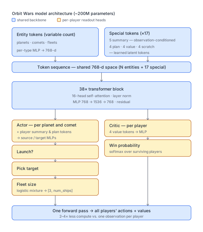
The input consisted of a number of relevant features for planets, comets, and fleets (e.g. radial and Euclidean position, velocity, encoded ship count) each projected separately via an MLP into a shared 768-dimensional representation. I included seventeen additional tokens: four player summary tokens, one global summary token, four actor plan tokens, four value tokens, and four scratch tokens. The player and global summary tokens were projected into the shared 768-dimensional representation from the observed features (total ships per player, total production per player, current step, etc.). The rest of the tokens used learned embeddings. Scratch tokens had no explicit purpose except to serve as a shared global workspace for the attention operation.

Once all tokens were projected into the shared embedding space, I fed them through a 38-block residual self-attention transformer with 16 attention heads per block, layer normalization, and MLPs with a 1536-dimensional hidden layer.

For each player, all planet/comet tokens were concatenated with that player’s summary and plan tokens before being passed through separate source and target MLPs. The source stream was projected down to a single Bernoulli logit per eligible source, sampled to decide whether or not to launch a fleet. Sources that decided to launch used a self-attention-like formulation for picking their target:

\[\frac{\mathbf{Q(source)} \cdot \mathbf{K(target)}}{\sqrt{d}}\]

Then, the selected target’s value vector $\mathbf{V(target)}$ was added into the source stream before being fed into a truncated discretized logistic mixture model with 8 mixture components to select the fleet size, in [3, num_ships].

I computed the critic output by feeding the value tokens through an MLP and then a softmax operation over all remaining players to estimate their win probability. I sampled all actions simultaneously, and computed the joint probability over all eligible sources for each player when calculating the PPO loss.

With this architecture, I could compute the actions for all players in a single forward pass, saving me 2-4x the compute over a standard one-observation-per-player approach.

Navigating submission constraints

I ran most early experiments using transformers with 1-5M parameters. Once I was confident that my implementation was working and the hyperparameters were reasonable, I began scaling up the model size. Each time I increased the number of parameters, the performance increased dramatically, so I continued scaling until I ran into two key limitations:

1. The submission only gets 1 second per turn plus 60 seconds of overage time, all running on a relatively slow CPU
2. The submission file size is capped at 100MiB

To run inference within the time limit, I used int8 quantization for the linear layers and capped the number of visible fleets, prioritizing the largest ones. This still wasn’t enough for about 8% of 4p games when the agent was assigned to a particularly slow CPU, so in those cases, I would continue playing normally until there was 1 second of overage time remaining, at which point I would switch over to using a much faster 5M model to play out the rest of the game. According to the learned critic, most games were already decided by the time the switchover occurred, and the 5M model was able to convert 100% of its winning positions.

To fit the 200M-parameter model into 100MiB, I used 4-bit NormalFloat codebook quantizationQLoRA: Efficient Finetuning of Quantized LLMs (Dettmers et al., 2023), which introduced the NF4 data type. with group size 128 and one fp16 scale for each group. Using this encoding, the quantized model could keep most of the original model’s performance, winning ~40% of the time against the non-quantized model in a head-to-head evaluation. In the interest of running an even larger model, I tried some 3-bit encoding methods, but the performance loss from 3-bit quantization outweighed the benefit of fitting a larger model, so I stopped at 200M parameters.

Environment rewrite

The included Python environment was too slow for RL, so I rewrote it in Rust. I used extensive parity tests against actual replays to verify that the simulation matched. Additionally, since actions were provided by the network as (source, target) pairs, I computed the required angles using the Rust code, avoiding the sun and other planets when possible. The Rust environment was also responsible for transforming a raw observation into the required model-compatible tensors. I preallocated and reused pinned memory buffers to minimize blocking CPU-GPU transfers, and ran many environments in parallel using multithreading.

Reinforcement learning with Proximal Policy Optimization

I elected to use PPOProximal Policy Optimization Algorithms (Schulman et al., 2017). instead of IMPALAIMPALA: Scalable Distributed Deep-RL with Importance Weighted Actor-Learner Architectures (Espeholt et al., 2018). because I appreciate its simplicity. Scaling PPO was quite straightforward, as I ran everything using distributed data parallel. I found that the throughput scaled linearly with both multi-GPU and multi-node training.

During training, I ran two-player and four-player games simultaneously, initially weighted evenly. The winner received a reward of +1 and the losers each received -1. I used pure self-play in order to maximize throughput. This was fine for two-player, but not ideal for four-player since the equilibrium dynamics are more complicated. I periodically evaluated the model head-to-head (using both 1v1 and 2v2 games) against the previous best checkpoint in order to measure progress. Once the model won >70% of its evaluation games, it replaced the previous best checkpoint. I added policy KL and cross-entropy value loss terms against the previous best checkpoint to help stabilize training, in addition to the standard GAE-λ advantage estimation,High-Dimensional Continuous Control Using Generalized Advantage Estimation (Schulman et al., 2015). clipped policy-gradient loss with advantage normalization, and entropy bonus.

I used frequent model checkpointing and occasional warm restarts to adjust hyperparameters for the larger models midway through a run. I tried training with an action mask that prevented the model from doing obviously silly things like launching its ships into the sun, but, much to my surprise, this made the trained model worse. I hypothesize that this may have been because excluding the mask forced the model to internally model more of the physics, which helped performance in other ways. I did end up bringing the mask back for some fine-tuning near the end of training and kept it during test time.

Hardware and performance

For hyperparameter tuning and early experiments, I trained using a single B200. Later, I ran larger-scale (25M-200M parameters) training experiments on an 8xB200 machine with 2048 parallel environments and 64-step rollouts. In the final days, I trained across four 8xB200 nodes with 8192 parallel environments. Training the 200M-parameter model ran at ~6.3M steps per GPU-hour (~110K tokens per GPU-second); training the final model therefore took ~2400 B200-hours.

Lessons learned

Handling stalling

I kept gamma, the future returns discount factor, at 1.0 (no discounting) so that the win probability value head could stay well-defined in four-player games. This resulted in a funny play-style where the model had no incentive to win now rather than later, so it would just acquire a ship lead and then stall for the rest of the game. While this behavior is fine at inference time, it was not ideal during training because it meant a lot of compute was wasted on already-decided games. Next time, I think I’ll try to include some sort of early truncation or surrender mechanism to improve the density of relevant states during training.

Balancing two-player and four-player modes

Throughout the competition, the top players were placed predominantly in two-player matches. I mistakenly assumed that this would continue through the end of the competition, so I prioritized two-player gameplay during the second half of training with a 90% two-player rate. However, after the final submission deadline, the four-player to two-player ratio shifted significantly to favor four-player games. Had I known in advance, I would have kept the two-player and four-player rates more balanced and added league-play against past checkpoints to help prevent strategic cycles and self-overfitting.

Better encoding the observation

Though the spirit of my approach involved mostly eschewing clever domain-specific tricks in favor of scaling the model size to the maximum, there is one trick I wish I had seen. Since fleets can’t change their flight path once they’ve launched, it’s possible to include all fleet information inside the per-planet features themselves instead of as separate entities. This provides two crucial benefits: the model no longer has to learn to predict where fleets are heading and, even more importantly, the model’s throughput is accelerated dramatically. Under my setup, most of the entities are fleets, meaning that a single state may require 200-300 entities, but using this encoding, that figure is dramatically reduced to at most 44 entities before the global tokens, resulting in a ~5x reduction in the average required compute per frame.

Self-play scaling laws

Throughout this competition, I had the sense that training a larger model for longer would produce a stronger final agent. This is what I had experienced in previous competitions, and was indeed borne out by a few small-scale experiments early on in Orbit Wars. However, after the final submission deadline had passed, I was curious to quantify more precisely: how much better is a larger model trained for longer?

To run the experiment, I trained a series of models from 1.5M parameters to 50M parameters using the same fixed set of hyperparameters that I had tuned during the competition. One notable exception was that I set the two-player rate to 0.75, so as to try and make the models somewhat comparable with the 200M model that had been trained with a mix of two-player rates 0.5 and 0.9. Additionally, I increased the batch size and number of training steps with the model size, so that as each successive model roughly doubled in size, I correspondingly doubled the batch size and total training steps.

To measure each model’s strength, I used the Bradley-Terry Elo rating system.Rank Analysis of Incomplete Block Designs: I. The Method of Paired Comparisons (Bradley & Terry, 1952). In this formulation, all ratings are relative, so I anchored the weakest final model at 0. The rating corresponds to the scaled log-odds, so an increase of $d$ Elo gives win odds of $10^{d/400} : 1$. For example, +100 Elo suggests 1.78x the odds (64% winrate), +200 Elo would be 3.16x the odds (76% winrate), and +400 Elo would be 10x the odds (91% winrate).

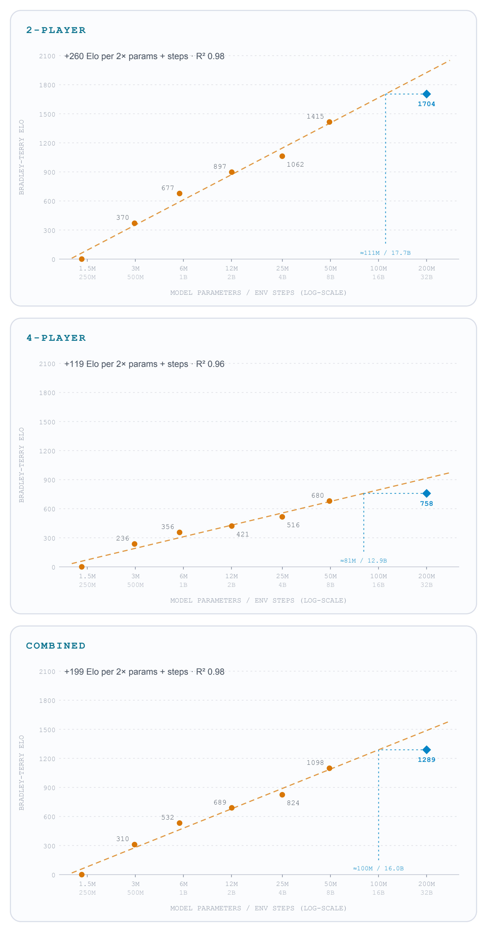
Final-checkpoint Elo vs model size. Params and training steps double together per rung; the dashed fit uses the six ladder runs only, and the blue diamond places the submitted 200M model on the same scale. The dotted guide reads off the ladder-recipe run its Elo would correspond to.

This result is already delightful: it shows that there is a remarkably predictive relationship between the size of the model, the number of steps it was trained for, and the resulting strength. This matches the precedent set by the Chinchilla Scaling Laws,Training Compute-Optimal Large Language Models (Hoffmann et al., 2022). but for self-play RL. I also noticed that the 200-million-parameter model trained for 15 billion steps fell around where the scaling laws would predict a ~100-million-parameter model trained for a comparable number of steps would lie. This made me further curious — what does the Elo chart look like over the course of training? And what is the relationship between the size of the model and the number of training steps required for it to reach its skill ceiling?

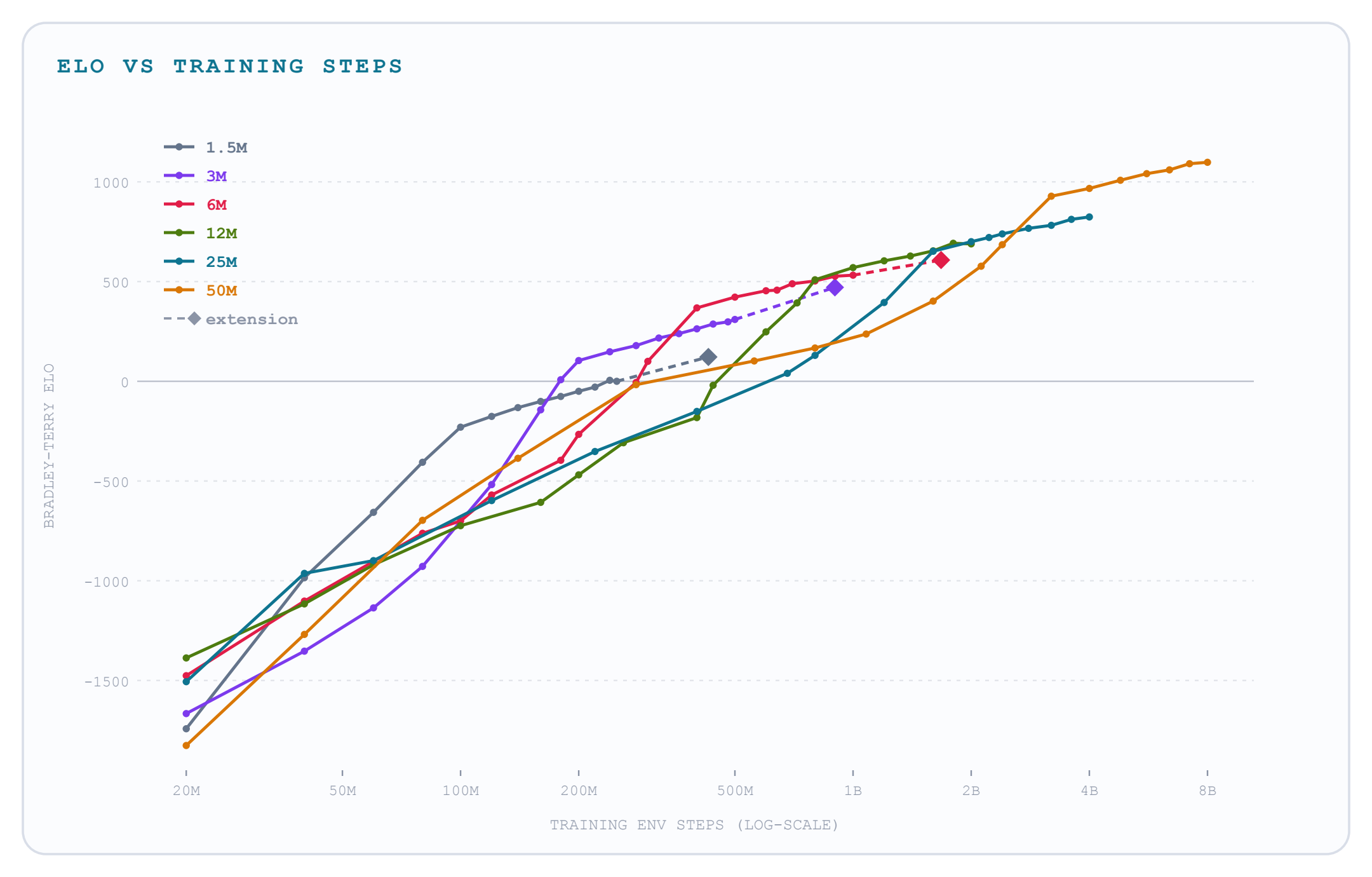
Combined (75% 2p / 25% 4p) Elo of each run’s checkpoints over training, measured head-to-head on the shared ladder scale. Dashed segments with diamond endpoints are floor-LR extensions past each recipe’s step budget. Even the smallest models continue to improve well past the point where I expected them to plateau.

Though it should be noted that the x-axis is in steps, not FLOPs, and the methodology is not identical, here again we see a relationship remarkably similar to the Chinchilla Scaling Laws:8 for any given compute budget, there exists some optimal model size. Too small, and you waste compute on a model whose performance is saturating. Too large, and you get a worse final model than you would have had you trained a smaller model on more steps instead. Additionally, I was surprised to see that I was not able to truly saturate even the smallest models I trained. Though it had been superseded by larger models at that point, even after 500M steps of training the 1.5M-parameter model was still steadily improving.

Closing thoughts

I want to thank the organizers at Kaggle, especially Bovard, for designing a delightful game and running a great competition. I had a wonderful time competing in Orbit Wars, and learned a ton along the way. It was as magical as ever to watch the agents learn: starting from random play and reaching their eventual superb skill level all with nothing but (a lot of) time spent playing the game. I look forward to the next one!